MIG Forensic 2020 – Synthèse
Taha Balkhi, Pierre-Louis Binachon, Thibaut Caillierez, Tristan Cotillard, Marguerite Dejean de La Bâtie, Louis Delmas, Anatole Hernot, Caroline Jeandat, Viviane Lesbre, François Mazé, Paul Meddeb, Victor Pachy, Alexis Sisca
This document is a brief summary of our notebooks and more generally of the work carried out during our project. For more information on how the algorithms work, the results obtained and the code of the algorithms, we invite the reader to refer to the notebooks related to each step of our work.
Context and presentation of the problem
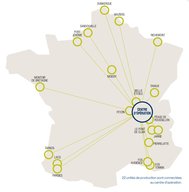
Air Liquide is a multinational industrial company specialized in industrial gases, particularly used in industry, healthcare, environment, and research. Air Liquide is active in 80 countries and employs about 67,000 people across 500 sites. As a global company, Air Liquide runs several industrial sites all around the world. Nowadays, 21 sites in France and some more in Italy are controlled remotely from a control center near Lyon.
As for any industrial group, and particularly since Air Liquide uses remote control, it is crucial for the group to be able to detect effectively and rapidly anomalies in the physical signals of their machines.
Since 2016, Air Liquide has been achieving its digital revolution with a plan called Smart Innovative Operations (SIO) in all his industries. The SIO program features four main components: SIO.Drive (remote control of the industrial sites), SIO.Optim (optimization of production to consume the least energy possible), SIO.Perform (analysis of the production performances) and SIO.Predict. SIO.Predict consists in achieving predictive maintenance. It aims to detect anomalies as soon as they appear in order to gain time and be able to repair the machine without impacting production, therefore avoiding economic losses. Indeed, shutting down a machine implies halting the customer's otherwise uninterrupted or limited supply. In Air Liquide Large Industries activity, customers are linked directly to Air Liquide’s factory using a pipeline. The production cannot tolerate any supply interruption. By detecting an anomaly right from its start, maintenance operations will be able to be done when the customer does not need the gases, thus making Air Liquide's maintenance process more secure and efficient. With a broader perspective, predictive maintenance allows the company to drastically reduce the cost of regular servicing: the machines are examined whenever an anomaly is detected and systematic checks, which force a complete stop of the system, therefore decrease.
To achieve this goal, SIO.Predict uses a software called PRiSM which defines a “normal” operating area thanks to the past normal data and which raises an alarm when the current parameters exit this area for a certain period of time (1st criterion). In addition, and even if the parameters stay within the desired area, PRiSM raises an alarm if one value varies too quickly (2nd criterion).
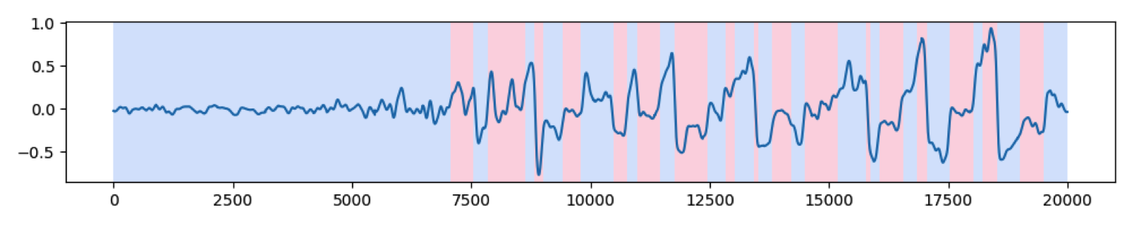
Despite its efficiency in detecting most anomalies, Air Liquide's implementation of PRiSM presents a specific flaw when parameters start to oscillate, whithin the normal range of values. These anomalies are rare but can cause major industrial issues. Slow oscillating anomalies are too slow to be considered an anomaly (2nd criterion) but their time period is still too short for the signal to stay out of the “normal” area for long enough (1st criterion). Resultantly, slow-oscillating — and often highly concerning — signals cannot be detected, or at least not before some time has passed.
This issue was observed on oil temperature measurement of a nitrogen compressor, due to a phenomenon called varnishing. When the temperature increases, little crystals form in the lubrication oil (due to impurities) and hold onto metallic parts, thereby preventing the oil from flowing. The lack of lubrication generates even stronger friction between metallic parts, thus increasing even more the temperature. The crystals eventually end up being detached by friction which re-establishes oil circulation and leads to a temperature decrease, hence the oscillating movement.
Both safety and economic gains could be achieved by developing an algorithm able to detect this type of oscillating anomalies. Solving this problem was the aim of our project, in which we developed a solution to the following question:
How can such oscillating anomalies recorded within a set of sensor data be detected with absolute certainty?
Our method
Forensic engineering
Let’s start by introducing Forensic Engineering. It can be defined as the retrospective investigation into industrial malfunctions and failures. The general purpose of a forensic engineering investigation is to locate one or several causes of failure in order to improve performance and avoid another accident. As mentioned, Air Liquide’s software, PRiSM, has got difficulties detecting the slow and frequent oscillations that may at a certain point lead to an industrial disaster with a risk of serious injuries and significant damage to the involved machines. Applying the Forensic approach, we collected various data from Air Liquide’s database and attempted to identify the features best suited to detecting the problem. We had sensor data spanning over 3 years and for 13 different physical values available to us. We chose one specific temperature as the variable of interest (main feature) for the different algorithms, since it was the one for which the issue to detect was most obvious due to the direct correlation between the varnishing phenomenon and the measured temperature. For some algorithms based on neural networks, other variables were required; these are explanatory variables (features that help the prediction of points and which must be as uncorrelated as possible).
The algorithms we programmed are classification algorithms: the data collected by Air Liquide may or may not correspond to an anomaly and are classified as such by our algorithms. Generally speaking, the objective of classification is to predict the class $y$ of an object $x$ as well as possible from observations on the latter. To help understand, let us describe for a moment the mathematical modelling of a generic classification problem.
Let $H$ be a measure space. To each point $X$ corresponds a label $Y \in \{0, 1\}$. The goal of statistical learning is to construct a function $$ h : H \to \{0,1\} $$ called a classifier, such that $h(X)$ best predicts the label of $X$.
Suppose that the pair $(X,Y)$ is derived from a draw according to a $P$ law. For a given classifier, the probability of misclassification is $L(h) = P(Y \neq h(X))$. We are therefore looking for a classifier which minimises $L(h)$.
If we know the law $P$, $L(h)$ is minimal for the Bayes classifier: $h_*(X) = \left\{ \begin{matrix} 1 \ \mbox{if} \ \mathbb{P}(Y=1 \mid X) \geq 1/2 \\ 0 \ \mbox{otherwise} \end{matrix} \right.$. In general we do not know the law $P$ but only a set of learning data $(X_i, Y_i)_{i=1, \cdots, n}$ following the law $P$. Our goal is therefore to construct from these learning data a classifier $\hat h$ which minimises $L(\hat h)-L(h_*)$.
Since the law $P$ is unknown, we instead calculate the empirical probability of misclassification: $$ L_n(h) = \frac{1}{n} \sum_{i=1}^n(\delta(Y_i \neq h(X_i)) $$
To a set $D \subset \Bbb F(H, \{0,1\})$ of classifiers we can associate the empirical risk minimisation classifier: $$ h_{\mathrm{min}}(D) \in \mathrm{argmin}\ _{h \in D} \ L_n(h) $$
Finally the quality of the approximation is: $$ L(h_{\mathrm{min}}(D)) - L(h_*) = \biggl (\min\ _{h \in D}\ L(h) - L(h_*)\biggr) + \biggl(L(h_{\mathrm{min}}(D)) - \min\ _{h \in D}\ L(h)\biggr) $$
The first term is the approximation error which can be reduced by expanding the set of classifiers studied. The second term is the estimation error, which is due to the fact that the empirical cost has been minimized and not the true probability of misclassification. This second term tends to increase with $D$.
The choice of $D$ is therefore important since there is a balance to strike between the approximation and estimation errors. This is why we have programmed different algorithms that explore different types of classifiers: the LSTM, the GAN, and the quantile regression classifier. This allows us, on the one hand to see if one type of classifier approximates better than another, and on the other hand to obtain a better result relative to specific metrics of interest (recall and precision, as defined later).
Our solution to the problem
The following sections present briefly the preprocessing step, as well as the five algorithms that we implemented. For more detail, please see the specific notebooks which gives more explanations, some graphical representations and the code for the following methods :
Preprocessing
More details available in the associated Notebook.
First we needed to preprocess our data, since raw data from Air Liquide are not usable as such by machine learning algorithms: they contain noise, outliers due to sensor faults, and long-term variations (for example the temperature follows the natural trend of the outside temperature induced by the seasons). We need to get rid of these issues in order to implement and use most of our algorithms.
The first step was thresholding. It consists in applying thresholds on the different features we selected (based on their relative correlation) that just replace every absurd value (error reports from the sensors which are constant known integers) with NaN values, NaN standing for “Not a Number”.
Then, comes the gap filling step. We filled all the gaps created either by the thresholding that induces NaNs but also by the missing measurements that occurred during the monitoring (we aim to obtain values at regular time intervals). Those gaps are replaced by points calculated using a linear regression for several reasons: their impact on the global appearance of the curve will be reduced by the other steps of the preprocessing, and this regression method is simple and is the least computation-intensive. Finally our customer did not want us to create values out of the blue and a linear approximation was close enough to reality to be acceptable.
The standardization step consists in highlighting the anomalies. To do that, we calculate the mean and the standard deviation of the signal on most of the normal phases of our training dataset and use these values to standardize the signal for every selected feature.
The signal remains full of noise and the gap filling step induced some abnormal intervals. Therefore, we need to find a function meeting a few requirements:
- Delete most of the noise
- Smooth the steep variations created by the gap filling
- Keep the global tendency of the signal
A compromise was found between the methods used and the bandwidth we wanted to work on in order to conciliate those requirements.
Now that high frequencies were erased from the spectrum, very low frequencies had to be cleaned out by the detrending step. This allowed us to keep only the frequencies we had to work on.
The signal — now preprocessed and cleared — could finally be fed into all of our algorithms, either for training them or for monitoring the machine. We strictly separated the test set from the train set, and kept a bit of data on the side for testing hyperparameter tuning. This is crucial for the machine learning algorithms that must not be tested on the data on which they were trained.
We decided to implement five different algorithms and then combined the results obtained using a voting system. The first two algorithms detect the oscillations (by analysing the signal’s structure): they are the Ruptures method and the EMD method.
Ruptures
More details available in the associated Notebook.
Ruptures is a Python library used to detect regime changes in a signal by returning a list of breakpoints. Only this library is not suitable for online operation. We decided to use the Pelt algorithm: its main attribute is that it doesn’t need to know in advance the number of breakpoints. We opted for optimizing the core of the Pelt algorithm so that it could adapt to online operation.
EMD
More details available in the associated Notebook.
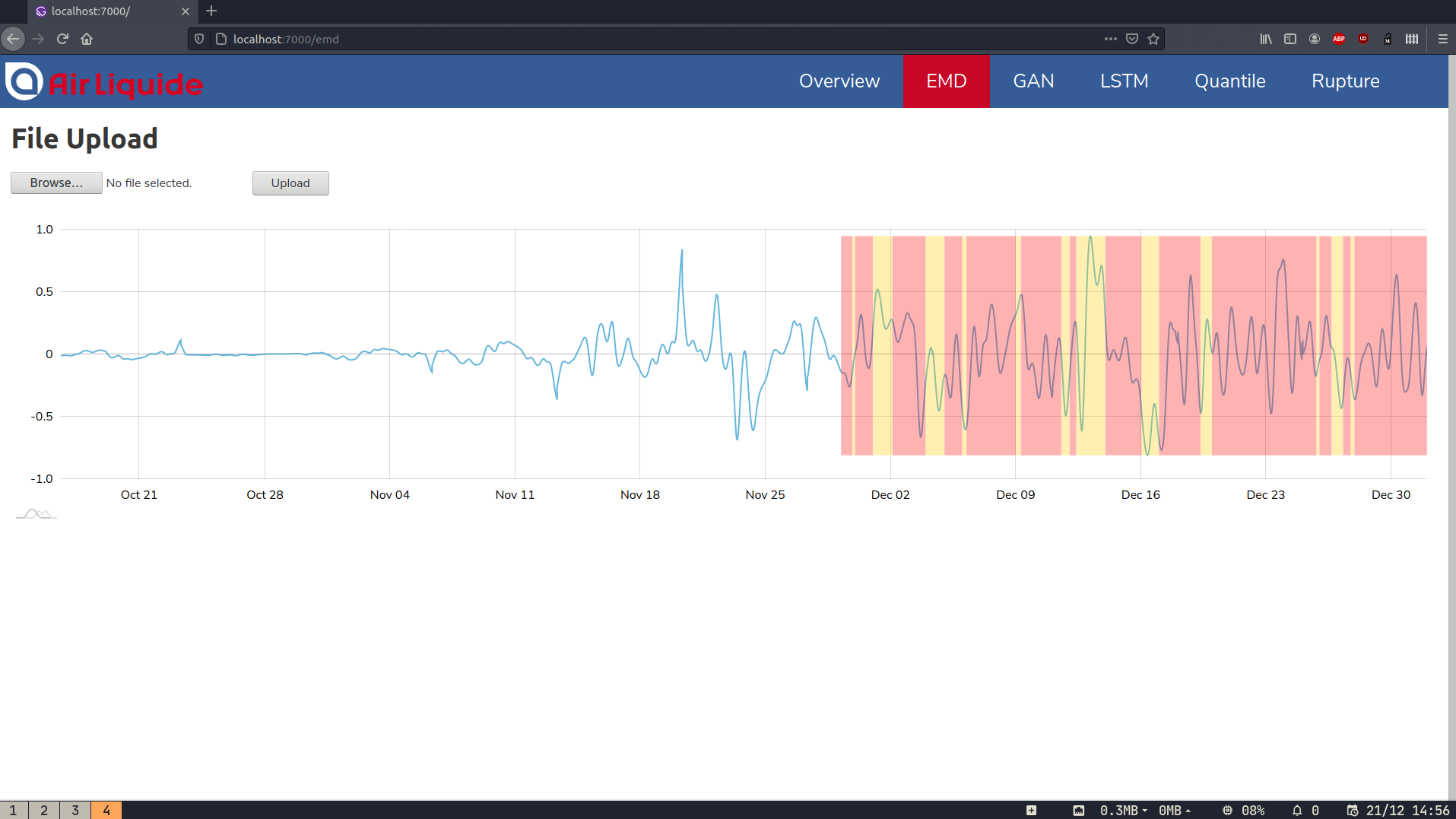
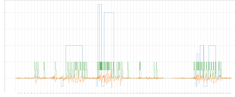
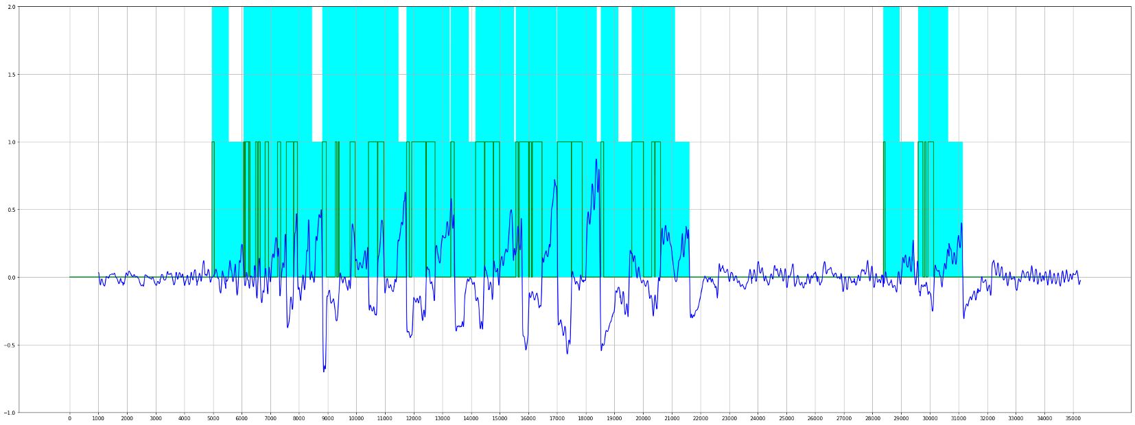
EMD (Empirical Mode Decomposition) is an empirical method of signal processing which decomposes a signal into IMFs (Intrinsic Mode Functions). A Hilbert transform of these IMFs allowed us to obtain their amplitude, and their instantaneous frequencies. We then noticed that the weak oscillations which caused the problem were quite obvious on these IMFs and that we could detect them using this method.
LSTM
More details available in the associated Notebook.
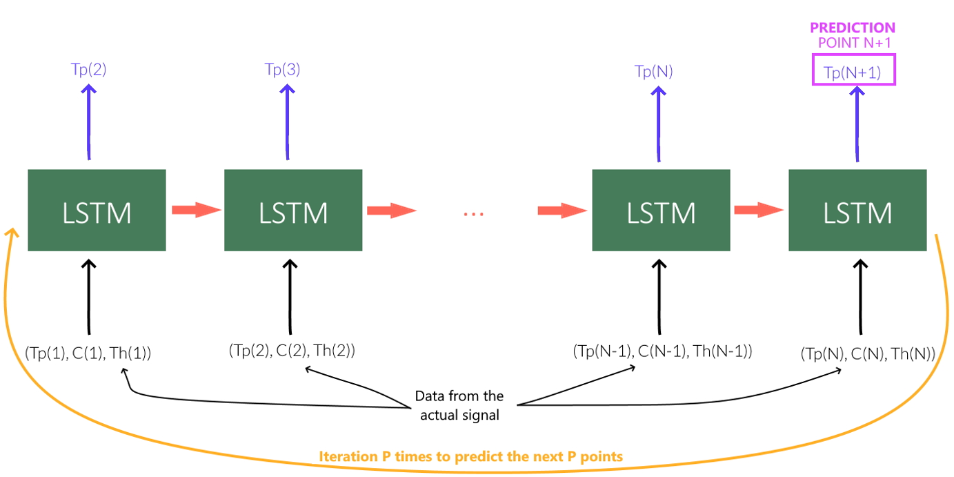
The Long and Short-Term Memory (LSTM) algorithm is a recurrent neural network that is able to predict the rest of the “Température palier étage 1” signal from the available signal history (past values) and that of other uncorrelated features (to maximize reliability) . When a signal is used as an input of the program, the output signal predicted for each point by the LSTM will be compared with the real one. If the two signals are different enough the input signal will be considered as abnormal.
Quantile regression
More details available in the associated Notebook.
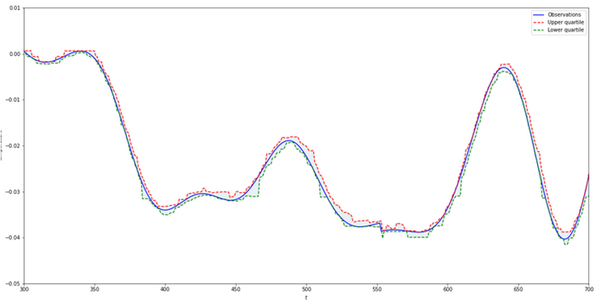
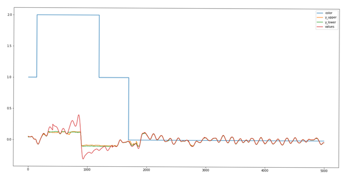
Quantile regression is a method of regression that works on the quantiles instead of the actual values. It is implemented through set learning using weak classifiers — trees — which, once assembled using gradient boosting, produce a single strong classifier. The advantage is that the method is way more robust than the standard least square regression against outliers. Indeed, on a large set of data, quantiles better depict the curve itself. Hence, with two quantiles we can predict an interval inside of which the values are expected to be found. And, like for the LSTM, if a bunch of values are outside of the predicted nominal range, an alarm will be raised.
GAN
More details available in the associated Notebook.
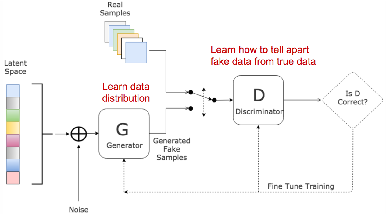
A GAN (Generative Adversarial Network) is an unsupervised neural network which is comprised of two neural networks competing to achieve the best results: the generator and the discriminator. The generator’s job is to generate believable fake data from random noise in order to fool the discriminator. The discriminator’s job is to discriminate between fake and real data being sent to it. This implies that, once shown erroneous data or some with visible anomalies, the discriminator will be able to detect it and raise an alarm.
Integration to the interface
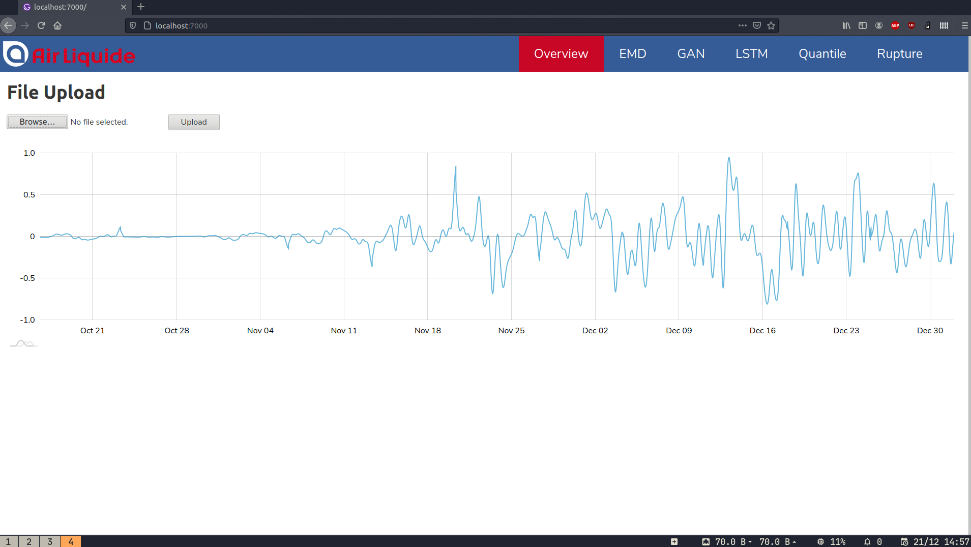
The interface is composed of several pages The main one displays the global alarm level depending on the system’s state obtained by the voting system (and shows its state at a given time with a month's history). Other pages are offered in order to see the individual results of the different algorithms.
Presentation and analysis of the results
To compare our algorithms and to have an idea of their performance, we used the precision and recall metrics. We focused on three variables:
- $T_p$ = the number of true positive anomalies (that are detected by the algorithm as anomalies and that are real problems)
- $F_p$ = the number of false positive anomalies (that are detected by the algorithm as anomalies but are not real problems)
- $F_n$ = the number of false negative anomalies (that are not detected by the algorithm as anomalies but are real problems)
The definitions of the recall and precision are:
- $\mbox{Recall} = \frac{T_p}{T_p + F_n}$
- $\mbox{Precision} = \frac{T_p}{T_p + F_p}$
- $\mathrm{F}_1\mbox{-Score} = \frac{2}{{1 \over \mathrm{Recall}} + {1 \over \mathrm{Precision}}}$
In other words, the recall quantifies the mistakes of an algorithm when not detecting an anomaly while the precision gives the percentage of true anomalies among all the anomalies detected.
We decided to privilege recall over precision because Air Liquide explicitly asked us to make sure all problems were detected. Since PRiSM already raises many false alarms, precision is less important but we still try to maximize it, if it does not impact the recall. Resultantly, recall, precision and F1_score (that combines the two) are key parameters to evaluate the performance of our algorithms.
Ruptures
The Ruptures method is quite different from the others: it is a rewriting of an already existing Python library, which automatically detects the changes of behaviour in a given curve. The modifications were aimed at drastically decreasing the computation time, which went from a few hours to a few seconds. This algorithm has a recall of 1.0 and an precision of 0.75, which results in a F1 score of 0.86.
EMD
The EMD method is not mathematically proven and is based on empirical observations. The algorithm detects the anomaly as soon as it happens, and the number of false positives is low, and mostly caused by gap filling. By analyzing the last 5,000 points every 10 minutes, the EMD method is optimally suited to real-time analysis and manages to raise relevant alarms. With a recall of 0.80 and an precision of 0.53, this algorithm has an F1 score of 0.64. The low recall in comparison with other algorithms is not a problem: it is mainly due to the alarms stopping during an anomaly, but the anomaly is always detected and, as the EMD works with other algorithms, there is no detection problem at all.
LSTM
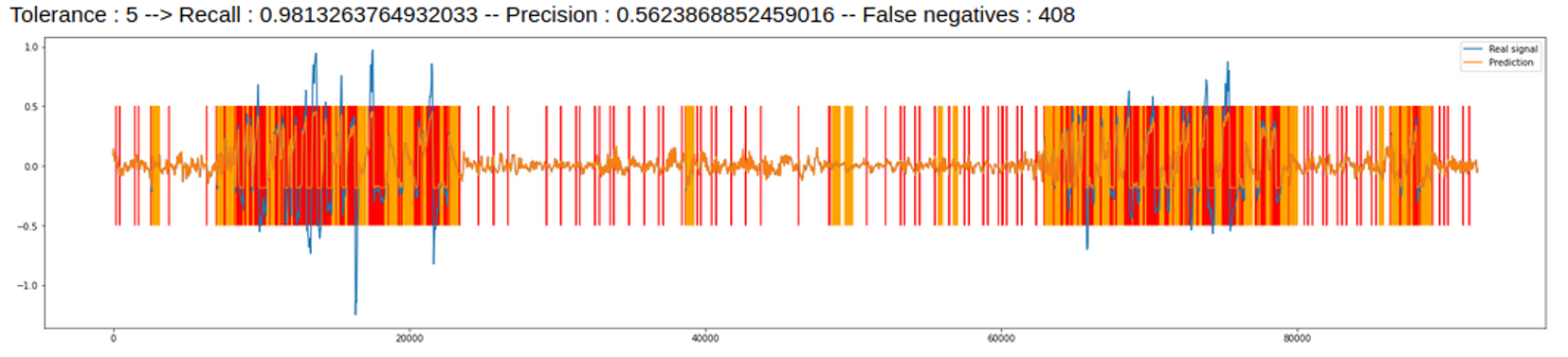
Once the hyperparameters and the tolerances of the algorithm are well chosen, the LSTM algorithm gives similar results to quantile regression. This may be justified by the fact that the two methods are actually close by their operation, unlike the other algorithms. The recall obtained is 0.98 while the precision and the F1 Score are respectively 0.56 and 0.71.
Quantile regression
The quantile regression method is fully mathematically proven. We get a recall of 0.99 and an precision of 0.58. Thus, the algorithm is very robust, as it does not miss real anomalies. As for the F1 Score, we obtain 0.73.
GAN
The final method, based on neural networks, is the most abstract machine learning solution and provides good performances. Indeed, the precision obtained is 0.67, the recall 0.98, and the F1 Score 0.80.
The voting system
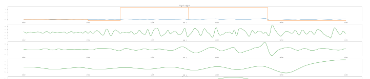
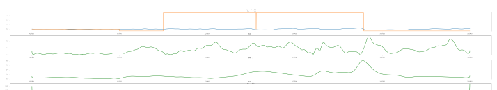
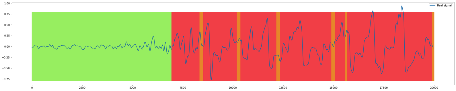
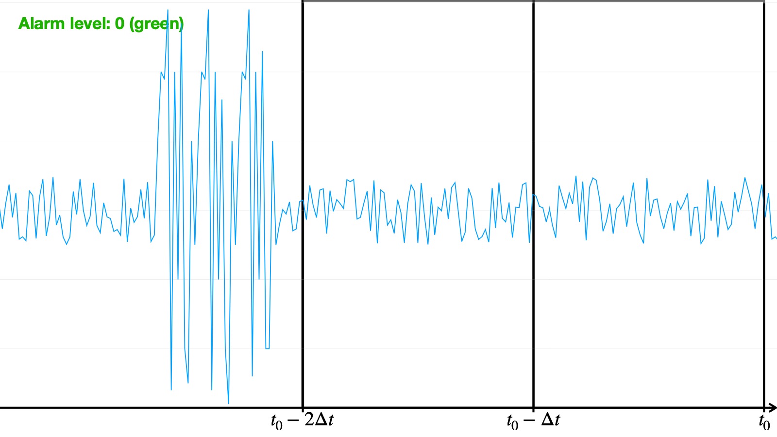
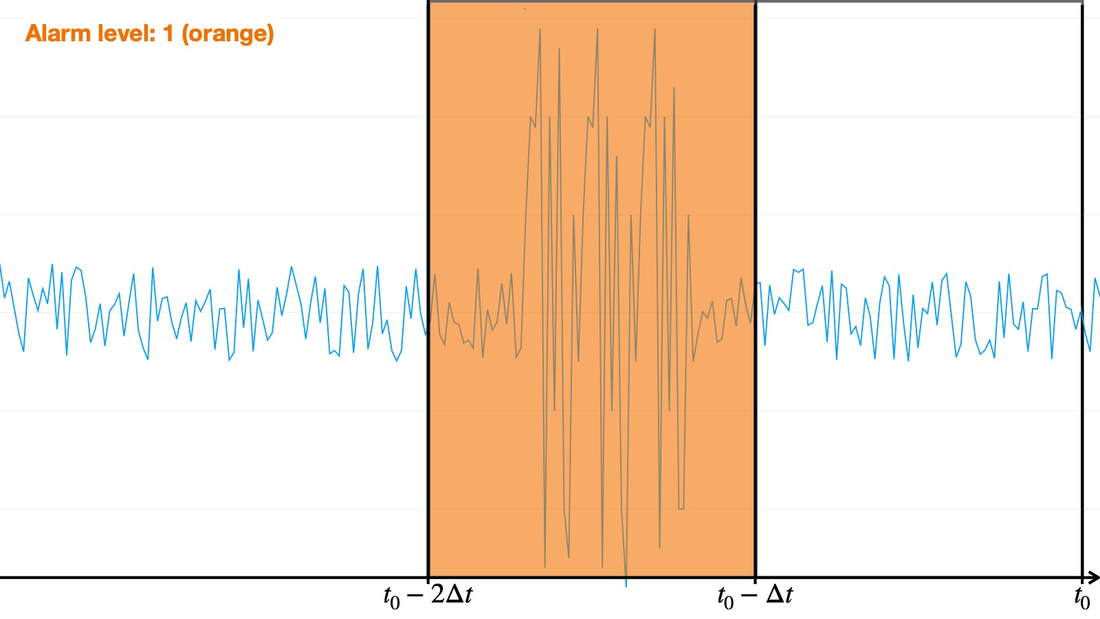
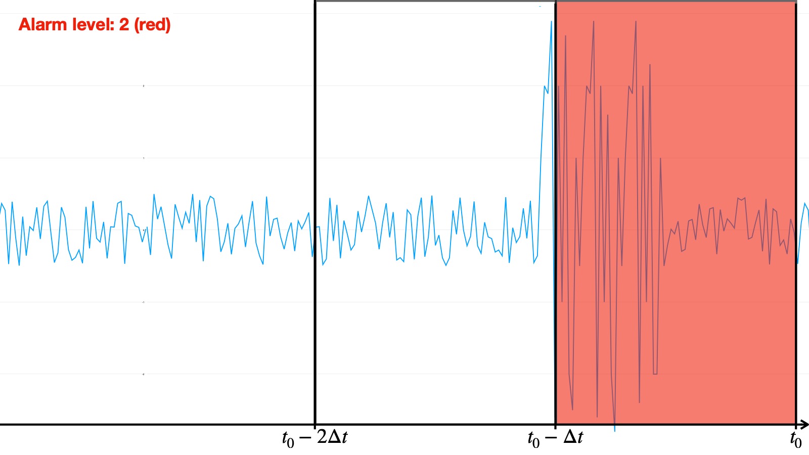
Given all these statistics on the algorithms, they must coordinate as a whole to detect the anomalies in an efficient way. In order to do that, we put into place a voting system which is based on three different types of alarms for each algorithm :
- Green: there is no anomaly
- Orange: there has been an anomaly recently
- Red: an anomaly is currently being detected by the algorithm
We then established a conditional voting system in order to give each algorithm a say in the final decision, taking into account the specificities of each algorithm — in particular, the different ways algorithms behave regarding the orange alerts: some often raise orange alarms within an actual anomaly whereas others almost only use red in an abnormal sequence. Consequently, an orange alarm raised by an algorithm of the first type is given more importance than an orange one from the second type. The final vote system is the following:
- If there are at least two red alarms, the probability that there is a real problem is very high, and we trigger the global alarm (red)
- Else, if there are at least three green alarms, we consider that there is no anomaly (green)
- Else, if the Ruptures-based algorithm or the GAN trigger a red alarm, we consult the three other algorithms, and if at least one of them is in orange alarm, we trigger the global alarm (red)
- Otherwise, we trigger the warning alarm (orange)
This way, we created a robust system of anomaly detection by prioritizing some algorithms that were more accurate and precise.
These performance statistics show that all five algorithms offer a recall close to 1 and precisions all above 0.53. These figures were presented to Air Liquide's data officer, who approved and was satisfied with the results.
Limitations of our solution and advice
Globally
The first limitation of this program is linked to the preprocessing of the data: all features are not preprocessed, only those which have been chosen after calculating the correlation matrix. The analysis of the correlation matrix revealed that only 5 were to be studied (plus the oil temperature for the LSTM). Furthermore to test our different algorithms we started the preprocessing by labelling the data, describing it as normal or not. This choice was done manually according to where we saw anomalies in the temperature data, therefore it is not perfect. This leads to some errors when we calculate the recall and precision of the algorithms: some rightfully find errors even if the labelling says the data has no problem. The general tendency is that our algorithms are more precise than the labelling.
Another limitation that we have encountered is the size of the dataset: since we had 3 years of data containing only 4 known anomalies available, this could lead to some underfitting - i.e. the deficient training of a machine learning algorithm due to the lack of training data - in the training of the predictors for the machine learning algorithms.
Finally, we tested our algorithms on the anomalies that were given to us; the algorithms detected all of them but it was impossible for us to test the former on all the possible anomalies that Air Liquide might have to face, given the limited size of the anomalous dataset we were provided with.
Another limitation is linked to the voting system. The latter was created by comparing the performances of every algorithm on a test dataset. Yet, the global system (including the vote) was not tested independently and thus may have been overfitted on the test data. To solve this issue, the global solution must be tested on a distinct dataset and the voting system ajusted if necessary.
Ruptures
Limitations
Considering the compromise found on the hyperparameters of the Pelt algorithm, the computation time for a partition of 10,000 points is more than reasonable, on the order of ten seconds. As Pelt's algorithmic complexity is linear, increasing the number of points would therefore not be a problem since we would then remain well below 10 minutes, the minimum time interval between two batches of data.
The Ruptures library offers the possibility of using different cost functions: we chose the quadratic cost function, which seemed to be the most suited for our problem (evaluation of the distance between two points). However, it would be necessary to examine whether there is a cost function which performs the task of detecting oscillations more optimally.
Advice
To obtain a more efficient algorithm which would then optimize the memory accesses and the cost calculation, we would have needed to:
- implement the Pelt algorithm as well as the cost function in a lower level language than Python, type C: this implementation was in progress but took us more time than expected, so we focused on the syntactic optimization of the Python version
- parallelize the computation of the cost function: this operation was not optimal in Python, but should save computation time as well as server load in C
However, we recommend running the Pelt algorithm as modified by us, with Python. Indeed, this version of the code remains very optimized and readable. In addition, it allows, through the Ruptures library written in Python, to use other cost functions than the one conventionally used (quadratic cost). Finally, even if we do not go through multi-processing to optimize the cost calculation, the calculation times are still very low. It is therefore a simple, optimized and readable version.
EMD
Limitations
- Empirical method with no mathematical proof.
- Partially-justified Hilbert transform (supposed to represent the instantaneous amplitude and frequency of the signal, here applied to already transformed signals) although IMFs are normally suited to this transformation.
- Statistical study on the module of IMFs and not the frequency, here again this is a purely empirical choice because this is where the most differences were noted.
- Establishment of a threshold whose value is mainly justified by its performance (studied by maximizing the F1 score).
- Inapplicable to other features or machines (it would be necessary to redo a statistical study on the transform of another signal). We only relied on the temperature.
- This method also reveals strange variations in the curve which are not for all that the oscillations, therefore a certain number of false positives.
Advice
- Improve the statistical method of determining the threshold value.
- Test other methods of analyzing MFIs (actually their Hilbert transformation).
- Interpreting the Hilbert spectrum
LSTM
Limitations
The LSTM algorithm raises an alarm when the difference between the real signal and the predicted one exceeds a certain threshold. Thus, it can be quite sensitive:
- Some anomalies are not detected. Or more precisely, within an anomaly, some parts of the signal can raise no alarm. Hence the importance to take the orange alarm into account, that indicates that a red alarm was raised in the near past.
- Even on a normal set, some red alarms are raised. If they don’t last and are not followed by an orange alert, they should not be taken into account (indeed, we have decided to only display the orange alert if the previous red one was lasting for long enough).
We only tested the algorithm on the limited data given to us: the precision could be improved by retraining on more data. However, as we only used normal data for the training, the algorithm should be able to detect anomalies different from oscillations. All signals that differ significantly from normal data can actually be detected.
We chose to train the LSTM on 3 features only. We didn’t try with all the features given. However, we tried with 6 features, as well as with only one. The results indicate that the choice of 3 features offers the best performance (see the annex to our notebook for more precision).
Advice
- Retraining the LSTM on more data could improve the precision and is necessary to adapt our algorithm on another machine
- The hyperparameters can be changed to improve the precision, or to decrease the number of false negatives
- At least 4 days of data must be given to our algorithm
Quantile regression
Limitations
The quantile prediction algorithm is known to converge only if the dataset it is trained on is infinite, hence leading to a loss of precision when using a finite dataset. Another issue of this algorithm is its sensibility to the hyperparameters: they were chosen according to the normal data in order to maximize the recall and F1_score, yet they can always be optimized.
Advice
- To have an adapted quantile predictor, it can also be useful to re-train it from time to time on new normal data. Another improvement of the efficiency is linked to the memory phenomenon: it has allowed us to increase the recall but decrease the precision. To adapt these parameters, the ratio used when comparing areas can be changed.
- With our algorithm, we were only working on the temperature of the 1st bearing, however to generalize this to another feature and therefore be able to supervise more the machines, the algorithm can be changed. For the quantile regression new predictors can be created and trained on other features to predict the interval for these new features.
GAN
As for the GAN algorithm, training was only performed on a single data series, thus resulting in a potential lack of generality when applying the model. As such, it is recommended that multiple features be included when re-training the model. Hyperparameter tuning was carried out empirically with little theoretical basis: despite appearing very suitable, it should be reconsidered in order to obtain the best fit. Additionally, testing was sparse and, although the results obtained were perfectly satisfactory, further testing shouldn't be ruled out to confirm the reliability of the model.
The voting system
The voting to determine the likeliest alarm level is performed on a basis of logical gates taking into account every algorithm's behaviour, notably regarding the meaning of an orange alert. We have decided to put all the algorithms on an equal footing for the vote but this choice remains arbitrary and we could consider implementing some weighting based on the algorithms' respective precision stats. Furthermore, a continuous alarm level ranging from 0 to 1 would be preferable to the discrete steps that are used to characterize the detected anomalies.
Special thanks
The entire group would like to warmly thank the following people, without whom this work would not have been possible.
Sébastien Travadel, who helped and guided us throughout the project,
Air Liquide, and particularly Frédéric Verpillat, who submitted this case study to us, and who made himself available to answer our questions,
Dănuț Matei and Luca Istrate, who helped us throughout the project and made it possible to integrate the solution in record time,
Tudor Cebere, George-André Silber, Benoît Gschwind, Philippe Blanc, for their support and help on technical points,
Nathalie Pitaval, who taught us how to organise the team work according to the principles of Lean Management,
Samuel Olampi & Franck Guarnieri.
Thank you all!